Alpha Diversity and Sequencing Depth
Following the phyloseq alpha diversity examples
Prune taxa
For this purposes I have taken the subset that includes samples only (i.e. excluded controls). Here we prune OTUS that are not present in any of the samples – BUT DON’T TRIM MORE THAN THAT! Many richness estimates are modeled on singletons and doubletons in the abundance data. You need to leave them in the dataset if you want a meaningful estimate.
physeq_prune <- prune_species(speciesSums(physeq1) > 0, physeq1)## Warning: 'prune_species' is deprecated.
## Use 'prune_taxa' instead.
## See help("Deprecated") and help("phyloseq-deprecated").
## Warning: 'speciesSums' is deprecated.
## Use 'taxa_sums' instead.
## See help("Deprecated") and help("phyloseq-deprecated").
Plot Examples
You can produce a range of alpha diversity estimates, however it is often slow to sped things up we’ll just use Chao1 and Shannon. Other include: Observed, ACE, Simpson, Fisher etc.
p = plot_richness(physeq_prune, measures=c("Chao1", "Shannon"))If you have a lot of samples it can look nicer to remove x axis and labels
p + theme(axis.title.x=element_blank(),
      axis.text.x=element_blank(),
      axis.ticks.x=element_blank())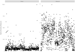
Colour samples by a variable
You may want to color your samples depending on a factor:
p = plot_richness(physeq_prune, measures=c("Chao1", "Shannon"), color = "Genus_Species")
p + theme(axis.title.x=element_blank(),
      axis.text.x=element_blank(),
      axis.ticks.x=element_blank())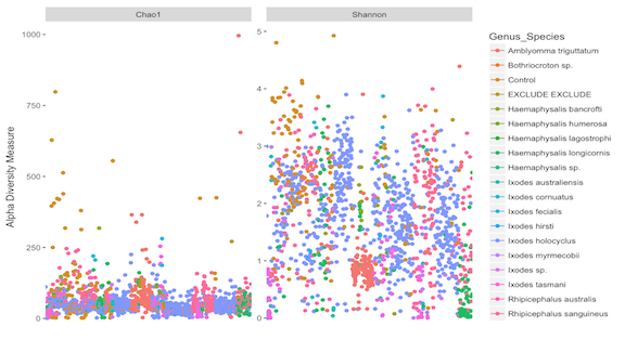
Separated by variable
You may also want to group samples based on a factor, which you can overlay ontop of the color factor.
p = plot_richness(physeq_prune, x="Host_common", measures=c("Chao1", "Shannon"), color = "Genus_Species")
p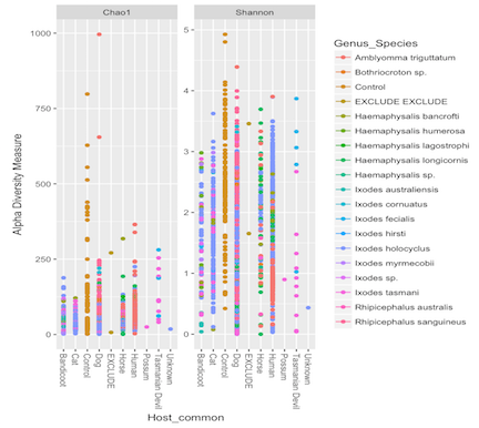
### Alpha diversity in microbiome
Additionally the microbiome package allows further options on alpha diversiy
This returns a table with selected diversity indicators
tab_alpha <- diversities(samples_only, index = "all")
head(tab_alpha)
inverse_simpson gini_simpson shannon fisher coverage
Sample1 8.312981 0.8797062 2.994656 14.381426 3
Sample2 2.956049 0.6617106 1.706885 4.509570 1
Sample3 9.076785 0.8898288 2.632313 4.932194 4
Sample4 5.562666 0.8202301 2.350704 6.644247 2
Sample5 4.418682 0.7736882 2.395877 5.964442 2
Sample6 2.961176 0.6622964 1.748629 8.315854 1
Vector and Waterborne Pathogens Research Group. 2018. S Egan.