Microbial Composition
Load libraries
library("phyloseq")
library("tidyverse")
library("readr")
library("ape")
library("plyr")
library("microbiome")
For large data sets, it is best to sub-set your data into smaller sections to first visualise what is going on and to ensure scripts are working.
For examples lets subset the original phyloseq object to just include Ixodes tasmani samples.
tasmani <- rownames(subset(meta(physeq1), Tick_Species == "tasmani"))
tasmani <- prune_samples(tasmani, physeq1)
nsamples(tasmani)
ntaxa(tasmani)
For aesthetic purposes it is best to prune the taxa to only include the more abundant taxa, have a play around with this figure - in this case we used 100, but you may want to adjust this depending on the number of taxa in the sampleset.
tasmanifilt = filter_taxa(tasmani, function(x) mean(x) > 100, TRUE)
ntaxa(tasmanifilt)
Abundance data
pcomp <- plot_composition(tasmanifilt,
                      taxonomic.level = "OTU",
                      sample.sort = "Host_common",
                      x.label = "Host_common") +
  guides(fill = guide_legend(ncol = 1))
pcomp
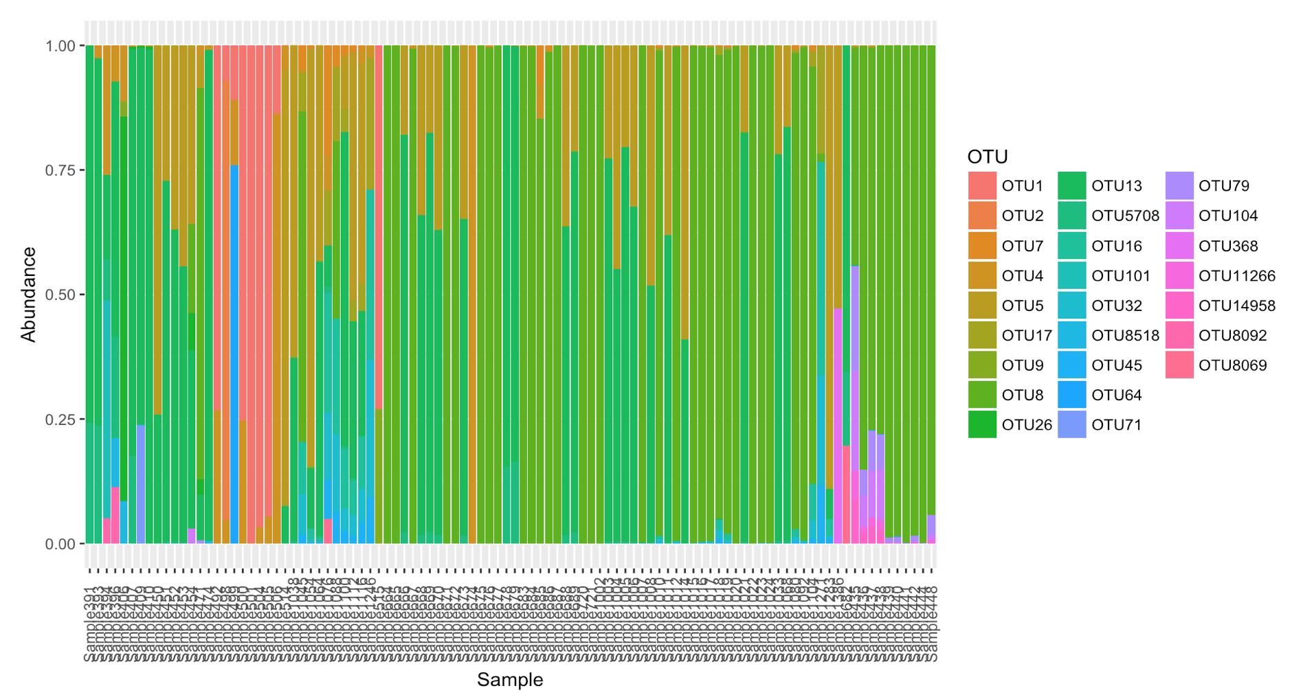
Compositional data
p <- plot_composition(tasmanifilt,
                      taxonomic.level = "OTU",
                      sample.sort = "Host_common",
                      x.label = "Host_commonr", transform = "compositional") +
  guides(fill = guide_legend(ncol = 3))
p
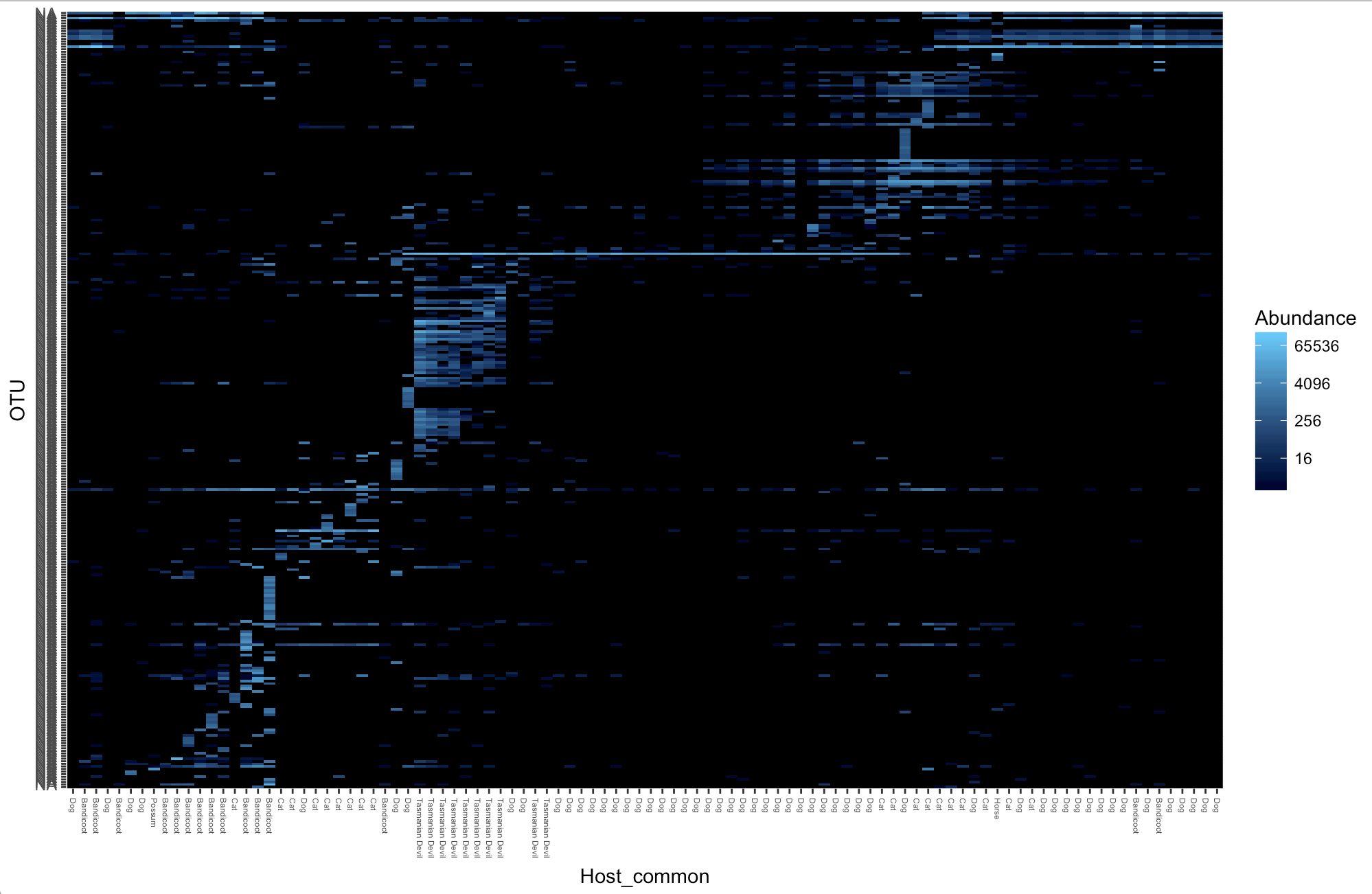
For Large datasets however this can often not be a useful way to show the microbial composition of the samples. Here we will use heat maps to show the relative abundance of taxa in samples
Heat maps
Here we use the Ixodes tasmani subset for quicker graphing
tasmani <- subset_samples(physeq1, Tick_Species== "tasmani")Then we will filter the top 300 OTUs
tasmani_300 <- prune_taxa(names(sort(taxa_sums(tasmani),TRUE)[1:300]), tasmani)
plot_heatmap(tasmani_300, sample.label="Host_common")
We can then subset a smaller set based on taxa
tasmani_Alphapro <- subset_taxa(tasmani, Class=="Alphaproteobacteria")
plot_heatmap(tasmani_Alphapro)
Vector and Waterborne Pathogens Research Group. 2018. S Egan.